Comparing a Basic OOP Query to
the New Category of Queries
Automatic Resolving of Objects Provides
Enhanced Flexibility in Searching Complex Data Structures
The same object model and its associated databases, used in the benchmarking tests (see the links below), are also utilized here to compare the properties of a basic OOP query with versions of queries employing the automatic resolving of objects, referred to here as the new category of database queries.
Performance Benchmarking on Many-to-Many (M:N) Relationships with Variations in Indexing and Sizes of Object Databases- Performance Benchmarking on Queries of a New Category with Variations in Indexing and Object Database Sizes
The object model comprises 12 Java classes, presented below in a text box and illustrated in the accompanying image.
The object model consists of 12 Java classes N1-N4, M1-M4 and S1-S4.
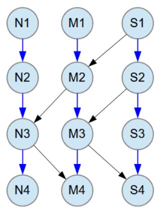
Blue arrow relationships between classes are M:N (many-to-many). All M:N relationships have 1-3 child objects at random.
Black arrow relationships between classes are M:1 (many-to-one).
The test object database contains 12 x 100K objects (where K = Thousand) and uses an indexing strategy that indexes all relationships between objects, as shown in the table below.
| RootDB Object Database in MariaDB | |||||
|---|---|---|---|---|---|
| Database Name | Number of Objects | Indexes | Creation Time (s) | Objects per Second | |
| ex100Krx | 12 x 100K | all relations | 1532 | 783 | |
Processor = AMD Ryzen 7 3700X, Disk Samsung SSD 860 EVO M.2 1TB
The following sections present query examples using the object database described in the table above. These examples include a comparison and discussion of a basic OOP query and the new category of queries, which leverage automatic resolving of objects based on their relationships within the object model.
Example of a Basic OOP Query
Query Variables and OOP Dot Notation Form the Foundation of RQL
Query variables (Qn) can be used to split a long search condition into multiple parts, enhancing readability and maintainability with shorter query expressions. For example, query variables are often used with the IN operator, where the left operand is a single or list reference field. The result objects of the query variable (the right operand of IN) define the parent (for a single reference field) or parents (for a list reference field). Essentially, the results of a query variable act as child objects, which are then used to automatically resolve their corresponding parent(s).
The source code for a basic OOP query, including the query variables Q1 and Q2, is shown below. The query is executed by calling the query.queryQ1Objects() method, which returns M1 objects and assigns them to the list variable listM1 of type List<M1>.
Additionally, the setParts(true) setting is applied to ensure that only the portions of objects involved in satisfying the search conditions are returned as query results. This means the returned results include only the specific parts of the objects that match the search criteria, rather than the complete data structures of the found M1 objects.
RQL query:
RootStore r5 = rdb.getRootStore("fi.rootrql.example9wrx.M1"); // M1
RootStore r6 = rdb.getRootStore("fi.rootrql.example9wrx.M2"); // M2
Query query =  Query.createQuery()
        .addQ1Query(r5,"(m2 IN (Q2))")
        .addQ2Query(r6,"(n3.m4.value = 770) MERGE (m3.s4.value = 50)")
        .setParts(true);
List<M1> listM1 = query.queryQ1Objects();
In this example, the query variable Q2 includes two search conditions defined relative to the M2 class (RootStore r5), with value conditions applied to classes M4 and S4. The search expression is "(n3.m4.value = 770) MERGE (m3.s4.value = 50)," where lowercase names like n3 and m4 represent reference fields pointing to their respective classes, N3 and M4. This notation, in which class names are capitalized and reference field names are written in lowercase, is consistently applied throughout the object models used here.
The condition for M4 is specified through the N3 class, while the condition for S4 is specified through the M3 class. The search results are merged in M2 using the MERGE operator, which functions as an AND operation. This ensures that only the results (data structures M2-N3-M4 and M2-M3-S4) from both search conditions that share the same M2 objects are included. The merged result represents the intersection of M2 objects, along with their associated query result data structures M2-N3-M4 and M2-M3-S4. This guarantees that the included data structures intersect in the same M2 objects, which are then used as the right operand for the IN operator in the search condition of the query variable Q1.
The query is illustrated in the picture below. The query variable Q2 is executed first, as it is referenced by the IN operator in the query variable Q1. The search results of its conditions, (n3.m4.value = 770) and (m3.s4.value = 50), are merged at M2. This merging is represented by red dashed lines connecting M2 to classes M4 and S4. Red X marks on classes M4 and S4 denote where the value conditions are set.
The query variable Q1 sets its search condition relative to the M1 class because it uses the RootStore variable r5. The search condition "(m2 IN (Q2))", searches for M1 objects whose reference list field m2 contains a reference to an M2 object present in the results of the query variable Q2. Note that Q2 returns M2 objects.
In the picture below, the Q1 query is represented by an indigo dashed line connecting classes M1 and M2. This illustrates how the database search is divided into two parts, as the query results at class M2, located within the data structure, are utilized and referenced by another query in the query variable Q1. The IN operator is highly effective for breaking down complex search expressions into multiple distinct query expressions, which are often easier for a programmer to write and read. It is worth noting that every search condition using the IN operator can also be rewritten as a strictly OOP-style query expression without using the IN operator.
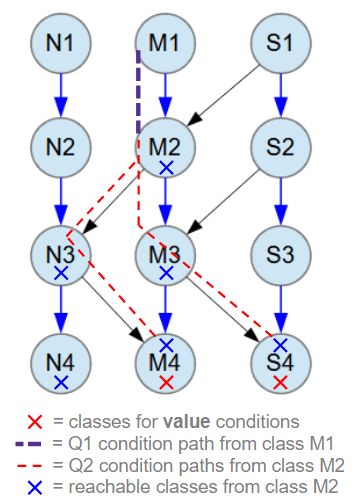
Blue arrow relationships between classes are M:N (many-to-many). All M:N relationships have 1-3 child objects at random.
Black arrow relationships between classes are M:1 (many-to-one).
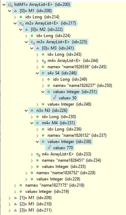
The query result contains four M1 objects, as shown in the picture below. The first M1 object is expanded in the debug view to reveal the field paths used in the search conditions. It can be verified that the s4 field of the M3 object references an S4 object with a field value of 50, and the m4 field of the N3 object references an M4 object with a field value of 770, as specified in the search conditions. Note that, due to the use of the setParts(true) setting, the results include only the specific parts of the M1 objects that satisfy the search conditions.
While the database search defined and executed as described above is straightforward and generally sufficient in terms of results, it lacks the flexibility to control the search through multiple paths within the data structure. For example, the search condition (n3.m4.value = 770) specifies a single path to M2. However, an alternative path, (m3.m4.value = 770), also exists, and both routes can be included in the search condition. Naturally, the resulting set of M1 objects is likely to differ from the results obtained with a single path.
In the basic OOP approach to RQL, allowing two paths involves using the OR operator to write the search condition as "(n3.m4.value = 770) OR (m3.m4.value = 770)". This approach works as expected, but RQL also offers an alternative method to achieve this, as discussed in the sections below.
Additionally, the returned results are limited to a single object type, restricting the query's versatility and efficiency. Enabling query results to include multiple class types simultaneously would not only enhance efficiency but also deliver an unprecedented programming experience for database queries.
To achieve these goals, a slightly different approach to writing and executing database queries can be adopted. This approach, referred to here as the new category of queries available in RQL, is demonstrated below by rewriting alternative versions of the above query using the conventions of the new query category.
Alternative Examples Using New Category Queries
RQL Offers a Highly Distributed Approach to Defining Search Conditions and Query Attributes
The First Alternative: Producing Identical Results
The purpose of the first alternative version is to return the same query results as in the previous example, but this time using the new category query features in RQL. RQL provides programmers with intuitive ways to define routes that are efficiently and automatically resolved. This resolving of objects can end at either internal objects or final root objects (located at the boundary) within a data structure stored in the database.
The source code for this alternative version is shown below. The query consists of four query variables: Q1, Q2, Q3, and Q4. The search conditions for the values 50 and 770 in classes S4 and M4 are defined in distinct query variables, Q3 and Q4, respectively. Each of these variables sets the resolveRoots attribute by calling its setter method, setQnResolveRoots, where n in Qn refers to the target query variable. The method's parameter specifies a list of classes used to resolve objects within the data structure. The order of classes in this list is not significant. For both query variables, the lists include the classes necessary to resolve objects up to class M2, which is an internal class in the data structure.
The resolving of objects up to class M2 is performed by the query variable Q2, which references both Q3 and Q4 in its search condition "(Q3 MERGE Q4)". However, it is not inherently clear to Q2 that it should use the automatic resolving method when executing its query expression, as the default behavior in RQL follows the basic OOP approach. To enable automatic resolving of objects, the resolveObjectModel attribute must be set to true for Q2, which is accomplished by calling the method setQ2ResolveObjectModel(true).
The execution of Q2 resolves the result objects of Q3 and Q4 up to class M2. Note that Q3 and Q4 return S4 and M4 objects, respectively, and their resolving path settings (defined by the resolveRoots attribute) are applied only when Q2 is executed. During its execution, Q2 merges the resolved M2 objects, which are obtained by resolving the query results of Q3 and Q4 (S4 and M4 objects). The resolved result consists solely of M2 objects, each including data structures extending to the associated S4 and M4 objects.
Ultimately, as in the previous example, the result objects should be M1 objects located at the boundary of the data structure, representing the final root objects. In practice, these root objects are those that cannot be further resolved using the object-resolving method.
After the execution of Q2, the result objects are M2 objects, and the next step is to resolve their corresponding M1 objects. This task is performed by the query variable Q1, which serves as the root for the entire query, directly utilizing Q2 and indirectly leveraging Q3 and Q4. The query expression for Q1, "(Q2)", is simply a reference to the already resolved query variable Q2 and may initially seem redundant. However, its functionality is clarified by setting the resolveRoots attribute, which specifies that the purpose is to resolve M1 objects for the given query expression.
The query is executed using query.queryQ1Objects(), initiating the complex set of query operations described above. However, it returns an empty result (and is therefore ignored) because Q1 is defined with the RootStore variable r6, which represents M2 objects instead of the resolved M1 objects. To obtain the resolved M1 objects, the RootStore variable r6 is used in the method call r6.transferObjectList("fi.rootrql.example9wrx.M1"), which retrieves the result as M1 objects. These objects are then assigned to the variable listM1, of type List<M1>.
Note that the setParts(true) setting is applied, ensuring that only the objects involved in satisfying the search conditions are returned as query results. In other words, the returned results include only the specific parts of the objects that match the search conditions, rather than the complete data structures of the found M1 objects.
RQL query:
RootStore r6 = rdb.getRootStore("fi.rootrql.example9wrx.M2"); // M2
RootStore r7 = rdb.getRootStore("fi.rootrql.example9wrx.M4"); // M4
RootStore r12 = rdb.getRootStore("fi.rootrql.example9wrx.S4"); // S4
Query query =  Query.createQuery()
        .addQ1Query(r6, "(Q2)")
        .setQ1ResolveRoots("fi.rootrql.example9wrx.M1")
        .addQ2Query(r3, "(Q3 MERGE Q4)")
        .setQ2ResolveObjectModel(true)
        .addQ3Query(r12,"(value = 50)")
        .setQ3ResolveRoots("fi.rootrql.example9wrx.M2",
    					   "fi.rootrql.example9wrx.M3")
        .addQ4Query(r7,"(value = 770)")
        .setQ4ResolveRoots("fi.rootrql.example9wrx.M2",
    					   "fi.rootrql.example9wrx.N3")
        .setParts(true);
query.queryQ1Objects();
List<M1> listM1 = r6.transferObjectList("fi.rootrql.example9wrx.M1");
The query defined by the source code above is illustrated in the picture below. The resolving paths used by the query variable Q2 are shown as red dashed lines for Q3 and orange dashed lines for Q4. The final step, resolving the root M1 objects from the M2 objects returned by Q2, is represented by an indigo dashed line.
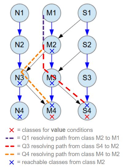
Blue arrow relationships between classes are M:N (many-to-many). All M:N relationships have 1-3 child objects at random.
Black arrow relationships between classes are M:1 (many-to-one).
The query result contains four M1 objects, identical to those returned by the basic OOP query above, as shown in the picture below. The first M1 object is expanded in the debug view to display the field paths used in the search conditions. It can be verified that the s4 field of the M3 object references an S4 object with a field value of 50, and the m4 field of the N3 object references an M4 object with a field value of 770, as specified in the search conditions.
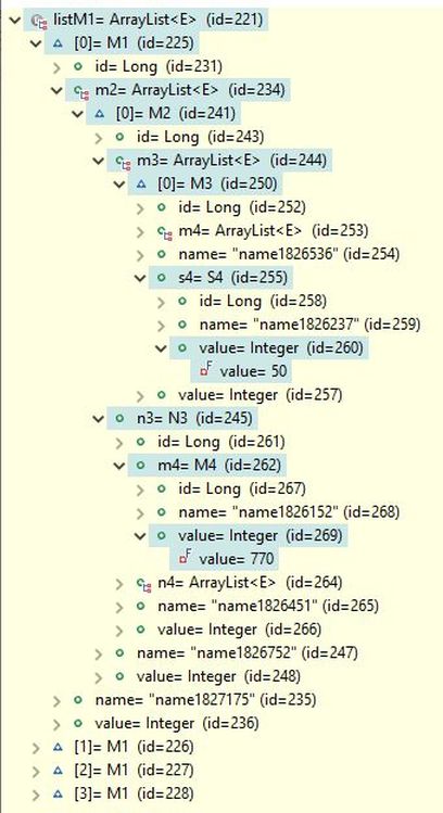
The above demonstrates a surprisingly agile alternative to the traditional approach of defining database queries, as exemplified by the previous basic OOP query. A key feature of this approach is its ability to define search criteria in a highly distributed manner within the data structure, while specifying allowed resolving paths separately as attribute data. This separation keeps the actual search conditions concise and straightforward. In fact, the allowed resolving paths, defined as query variable attributes, become a central element of the entire database query definition.
The Second Alternative: Expanding the Scope of Results
In the first alternative above, the returned results are limited to a single object type, specifically M1 objects. However, the automatic resolving of objects can be configured to resolve root objects of multiple types simultaneously.
This is accomplished by extending the resolveRoots attribute list of Q1 with additional classes to be included in the automatic object resolving process. This approach ensures highly efficient execution, as only the classes that the programmer specifically needs in the results and identifies as potential root objects participate in the resolving process.
The source code below presents a revised version of the RQL query where the resolveRoots attribute is extended to include the class S1, enabling Q1 to resolve both M1 and S1 classes. However, Q1 still returns an empty result (and is therefore ignored) because it is defined with the RootStore variable r6, which represents M2 objects instead of the resolved M1 and S1 objects. To retrieve the resolved M1 and S1 objects, the RootStore variable r6 is used to call the transferObjectList method twice, once for each class, M1 and S1. The retrieved M1 and S1 objects are then assigned to the variables listM1 and listS1, of types List<M1> and List<S1>, respectively.
RQL query:
RootStore r6 = rdb.getRootStore("fi.rootrql.example9wrx.M2"); // M2
RootStore r7 = rdb.getRootStore("fi.rootrql.example9wrx.M4"); // M4
RootStore r12 = rdb.getRootStore("fi.rootrql.example9wrx.S4"); // S4
Query query =  Query.createQuery()
        .addQ1Query(r6, "(Q2)")
        .setQ1ResolveRoots("fi.rootrql.example9wrx.M1",
                           "fi.rootrql.example9wrx.S1")
        .addQ2Query(r3, "(Q3 MERGE Q4)")
        .setQ2ResolveObjectModel(true)
        .addQ3Query(r12,"(value = 50)")
        .setQ3ResolveRoots("fi.rootrql.example9wrx.M2",
    					   "fi.rootrql.example9wrx.M3")
        .addQ4Query(r7,"(value = 770)")
        .setQ4ResolveRoots("fi.rootrql.example9wrx.M2",
    					   "fi.rootrql.example9wrx.N3")
        .setParts(true);
query.queryQ1Objects();
List<M1> listM1 = r6.transferObjectList("fi.rootrql.example9wrx.M1");
List<S1> listS1 = r6.transferObjectList("fi.rootrql.example9wrx.S1");
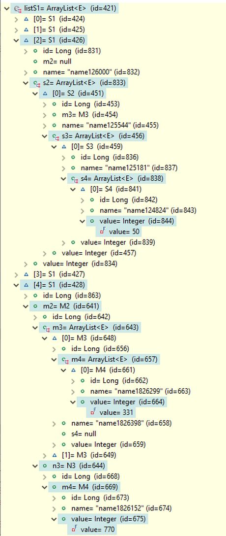
The query result contains four M1 objects, identical to those returned in the previous query examples, along with one S1 object, as shown in the picture below. The first object in listM1 and the only S1 object are expanded in the debug view to display the field paths used in the search conditions. It can be verified that the s4 field of the M3 object references an S4 object with a field value of 50, and the m4 field of the N3 object references an M4 object with a field value of 770, as specified in the search conditions. Notably, the first M1 object and the only S1 object both refer to the same M2 object with id=322 through their m2 reference fields - a list of references in M1 and a single reference field in S1 - indicating that they share the same M2 object.
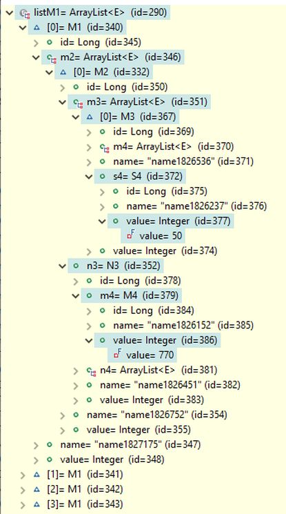
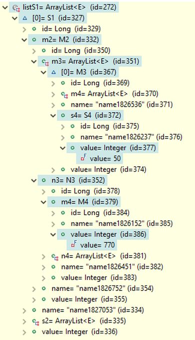
The above query can be slightly modified for cases where the programmer requires all classes available in the object model to be resolved. To enable this type of automatic resolving of objects, the resolveObjectModel attribute must be set to true for Q1, which is done by calling the method setQ1ResolveObjectModel(true). The source code for this version is shown below.
Although this version may be slightly less efficient than the one where the exact classes are explicitly listed for resolving, the performance difference is generally negligible. However, despite the convenience of not listing classes for resolving, the programmer must still know the specific classes when calling the transferObjectList method to retrieve the corresponding result objects.
RQL query:
RootStore r6 = rdb.getRootStore("fi.rootrql.example9wrx.M2"); // M2
RootStore r7 = rdb.getRootStore("fi.rootrql.example9wrx.M4"); // M4
RootStore r12 = rdb.getRootStore("fi.rootrql.example9wrx.S4"); // S4
Query query =  Query.createQuery()
        .addQ1Query(r6, "(Q2)")
        .setQ1ResolveObjectModel(true)
        .addQ2Query(r3, "(Q3 MERGE Q4)")
        .setQ2ResolveObjectModel(true)
        .addQ3Query(r12,"(value = 50)")
        .setQ3ResolveRoots("fi.rootrql.example9wrx.M2",
    					   "fi.rootrql.example9wrx.M3")
        .addQ4Query(r7,"(value = 770)")
        .setQ4ResolveRoots("fi.rootrql.example9wrx.M2",
    					   "fi.rootrql.example9wrx.N3")
        .setParts(true);
query.queryQ1Objects();
List<M1> listM1 = r6.transferObjectList("fi.rootrql.example9wrx.M1");
List<S1> listS1 = r6.transferObjectList("fi.rootrql.example9wrx.S1");
In this case, the results are identical to the previous version because the classes M1 and S1, the only possible parent classes for M2, were also included in that version. Note that the resolveObjectModel attribute is set to true for a query variable in two use cases. The first is when the object-resolving method is used to resolve objects up to the root objects (those at the boundary of the data structure), as demonstrated with Q1 above. The second is when a query variable contains a query expression consisting of references to other query variables with object-resolving definitions, as shown with Q2 above. In this latter case, the resolveObjectModel attribute indicates that the query variable should execute the resolving definitions for the referenced query variables and then evaluate its logical expression based on their resolved results.
The Third Alternative: Expanding Routes Within the Data Structure
To demonstrate the agility and flexibility of queries when the object-resolving method is applied, the RQL query from the previous example is enhanced to allow two routes from M4 to M2, as illustrated in the picture below. Previously, there was only a single route, M4 → N3 → M2. Now, an additional route, M4 → M3 → M2, has been introduced, as indicated by the orange dashed lines in the picture.
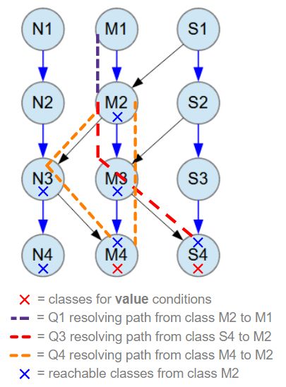
Blue arrow relationships between classes are M:N (many-to-many). All M:N relationships have 1-3 child objects at random.
Black arrow relationships between classes are M:1 (many-to-one).
Previously, the source code included two classes, N3 and M2, in the value list of the resolveRoots attribute for query variable Q4, which had the search condition (value = 770) for M4 objects. The new resolving route through M3 is added by simply enhancing the resolveRoots attribute list with the M3 class. The updated source code is provided below. Note that the search condition of Q4 has been relaxed to (value = 770) OR (value = 331) because the database contains no M3 objects referencing M4 objects with the previous condition.
RQL query:
RootStore r6 = rdb.getRootStore("fi.rootrql.example9wrx.M2"); // M2
RootStore r7 = rdb.getRootStore("fi.rootrql.example9wrx.M4"); // M4
RootStore r12 = rdb.getRootStore("fi.rootrql.example9wrx.S4"); // S4
Query query =  Query.createQuery()
        .addQ1Query(r6, "(Q2)")
        .setQ1ResolveRoots("fi.rootrql.example9wrx.M1",
                           "fi.rootrql.example9wrx.S1")
        .addQ2Query(r3, "(Q3 MERGE Q4)")
        .setQ2ResolveObjectModel(true)
        .addQ3Query(r12,"(value = 50)")
        .setQ3ResolveRoots("fi.rootrql.example9wrx.M2",
    					   "fi.rootrql.example9wrx.M3")
        .addQ4Query(r7,"(value = 770) OR (value = 331)")
        .setQ4ResolveRoots("fi.rootrql.example9wrx.M2",
                           "fi.rootrql.example9wrx.M3",
    					   "fi.rootrql.example9wrx.N3")
        .setParts(true);
query.queryQ1Objects();
List<M1> listM1 = r6.transferObjectList("fi.rootrql.example9wrx.M1");
List<S1> listS1 = r6.transferObjectList("fi.rootrql.example9wrx.S1");
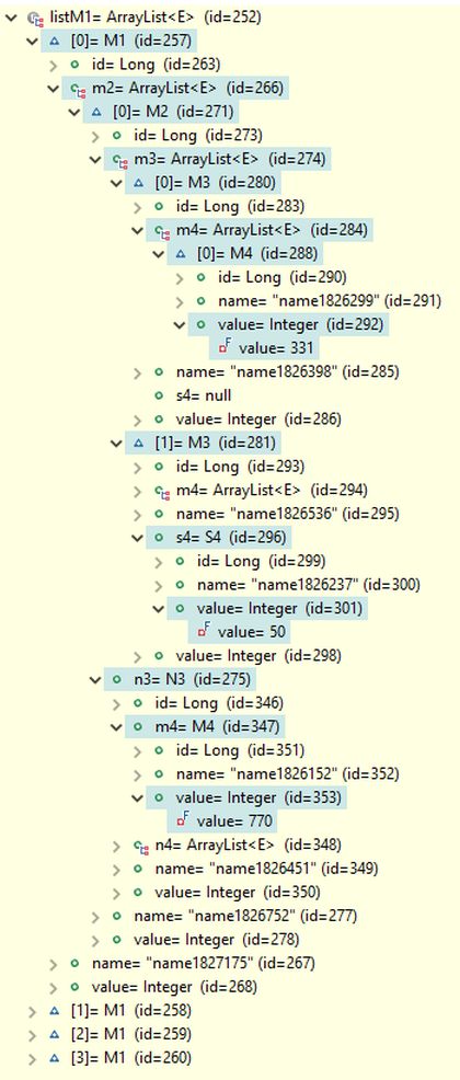
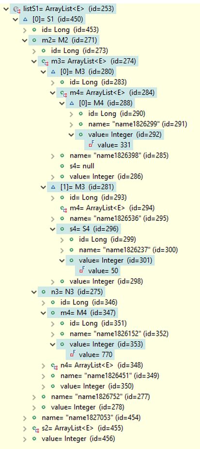
The query result includes four M1 objects and one S1 object, as shown in the picture below. The first object in listM1 and the only S1 object are expanded in the debug view to display the field paths used in the search conditions. All search conditions - (value = 770), (value = 331), and (value = 50) - are found as expected in the M4 and S4 objects. Additionally, the debug view confirms that the route from M3 to M4 is utilized, and the corresponding M4 object contains the expected value 331.
As mentioned, the key feature of this approach is its ability to define search criteria in a highly distributed manner within the data structure, while specifying the allowed resolving paths separately as attribute data. This separation ensures that the actual search conditions remain concise and straightforward.
The Fourth Alternative: Allow All Routes Within the Data Structure
When the task is to search for objects located at the boundary of the data structure (the ultimate root objects) without the need to restrict resolving to specific routes or calculate intermediate search results within the data structure, the object-resolving process can be allowed to utilize all available routes in the object model.
In the source code below, the same search conditions as in the previous third alternative are applied to objects of classes M4 and S4. However, instead of specifying the allowed routes in the resolveRoots attribute, the resolveObjectModel attribute is set to true for the query conditions at classes M4 and S4. This ensures that all routes in the object model are automatically considered during the process of resolving the root objects. For programmers, this provides a highly convenient method for writing queries, as the selection of routes through the data structure is handled automatically.
The query variable Q1 contains the query expression that is evaluated first when the database query is initiated by calling the method query.queryQ1Objects(). Its query expression, "(Q3 MERGE Q4)", references the query variables Q3 and Q4, where their respective value conditions, "(value = 50)" and "(value = 770) OR (value = 331)", are defined.
RQL query:
RootStore r5 = rdb.getRootStore("fi.rootrql.example9wrx.M1"); // M1
RootStore r7 = rdb.getRootStore("fi.rootrql.example9wrx.M4"); // M4
RootStore r12 = rdb.getRootStore("fi.rootrql.example9wrx.S4"); // S4

Query query =  Query.createQuery()
        .addQ1Query(r5, "(Q3 MERGE Q4)") //M1
        .setQ1ResolveObjectModel(true)
        .addQ3Query(r12,"(value = 50)")  //S4
        .setQ3ResolveObjectModel(true)
        .addQ4Query(r7,"(value = 770) OR (value = 331)") //M4
        .setQ4ResolveObjectModel(true)
        .setParts(true);
List<M1> listM1 = query.queryQ1Objects();
List<S1> listS1 = r5.transferObjectList("fi.rootrql.example9wrx.S1");
When Q1 is executed, the database is queried using these conditions, and the results are the matching S4 and M4 objects. The execution of Q3 and Q4 then continues by automatically resolving the root objects for these result objects, navigating through the data structure along the routes defined in the object model. For M4 objects, the possible root objects are N1, M1, and S1, as visualized by the orange dashed lines in the picture below. For S4 objects, the possible root objects are limited to M1 and S4, indicated by the red dashed lines.
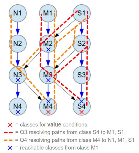
Blue arrow relationships between classes are M:N (many-to-many). All M:N relationships have 1-3 child objects at random.
Black arrow relationships between classes are M:1 (many-to-one).
Finally, Q1 performs the MERGE operation on the result objects from Q3 and Q4 to resolve the ultimate root objects. The method query.queryQ1Objects() is executed on the query variable Q1 and returns the resolved root objects of type M1. This is because Q1 is defined with the RootStore variable r5, which is bound to M1 objects. The returned M1 objects are then assigned to the variable listM1 of type List<M1>.
S1 result objects are retrieved by calling the method r5.transferObjectList("fi.rootrql.example9wrx.S1") and are assigned to the variable listS1 of type List<S1>. While N1 result objects could also be retrieved by calling the transferObjectList method with their class name "fi.rootrql.example9wrx.N1", this is not done. The MERGE operation acts as an AND operation on the root objects found by Q3 and Q4. According to the object model, S4 objects lack a route to N1 objects. Therefore, the resolved root objects for the found S4 objects cannot include any N1 object.
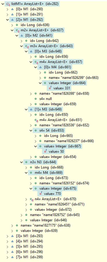
The query result includes eight M1 objects and thirteen S1 objects. The found M1 objects are listed in the picture below, but only the first five S1 objects are shown to limit the picture's height. In the debug view, the third object in listM1 is expanded, while in listS1, the third and fifth objects are expanded. These debug views display the field paths used in the search conditions. All search conditions—(value = 770), (value = 331), and (value = 50)—are found as expected in the M4 and S4 objects.
Furthermore, the debug view confirms that the routes M1 - M2 - M3 - M4, M1 - M2 - N3 - M4, S1 - M2 - N3 - M4, S1 - S2 - S3 - S4, and S1 - M2 - M3 - M4 are among the results. The searched objects along these routes have the required values as specified in the search conditions.
The automatic selection of routes to root objects does have a slight negative impact on execution performance, but it is not as significant as one might expect. As a result, this approach can be widely recommended for most use cases. Optimization of object model routes can be reserved for scenarios where the number of objects is very large or even exceptionally large.
Summary
The strength of this new category of database searches lies in its flexibility to set multiple search conditions anywhere within the data structures, combined with the ability to define allowed routes in the resolveRoots attribute to guide automatic object resolving. Alternatively, setting the resolveObjectModel attribute to true enables fully automatic route selection based on the database's object model.
These attributes, together with the search conditions, collectively define queries for complex data structures in databases. Even with versatile conditions, the queries are automatically and efficiently resolved, enabling the discovery of root objects from multiple classes along with their associated data structures. This separation ensures that the search conditions remain concise and straightforward. Indeed, the allowed resolving routes, specified as query variable attributes, become a central component of the entire database query definition.
Links to other pages on this site.
- Performance Comparison Many-to-Many (M:N) Relationships with Indexing
- Performance Comparison Many-to-Many (M:N) Relationships without Indexing
- Performance Benchmarking on Many-to-Many (M:N) Relationships with Variations in Indexing and Sizes of Object Databases: Performance Comparison with Multiple Query Conditions in an Object Hierarchy
- Performance Benchmarking on Queries of a New Category with Variations in Indexing and Object Database Sizes
Performance Comparison with Multiple Query Conditions in an Object Hierarchy - RootDB, Technical Features
- RootDB and RQL, Home
Page content © 2025

Contact us:
